
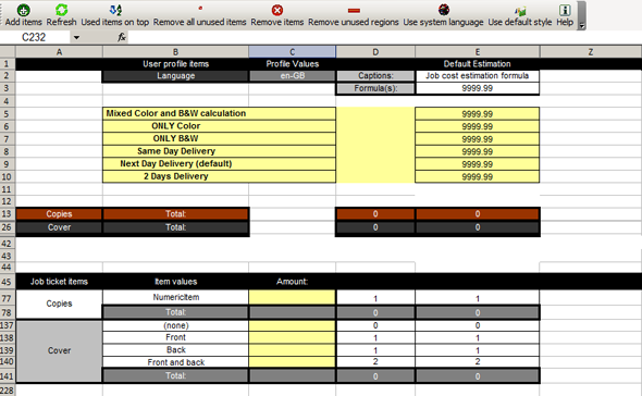
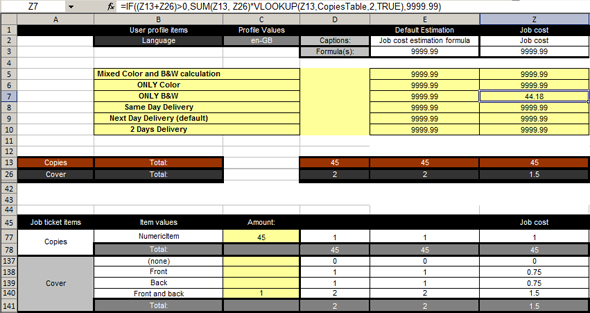
By default, a number of formulas are available. You can define custom formulas in the columns next to the default formulas up to and including column Z. Each column can contain one formula. Each column contains all information for one formula:
The name and the calculated result of the formula.
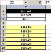
The result of the formula is shown in row 3.
The calculation for the formula.
The formula can use one of the default calculations, or a custom calculation.
The calculation collects its values from the concerning column in the result table.
The result table collects the values for all job ticket items from the concerning column in the job ticket table.
The job ticket table receives its values from the current job ticket definition.
It is recommended that you do not remove the default formulas.
The required [Job ticket items] for the new formula must be available.
In this procedure a complete new formula is created in column Z of the worksheet "CostSheet". The new formula is based on two [Job ticket items]: [Copies] and [Cover]. In this example, the data of the formula in column E is used as starting point for the formula in column Z.
The formulas and formatting of column E are copied into column Z. The cell references are automatically adjusted.
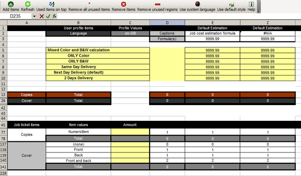
The formula names in row 1 are displayed in the [PRISMAaccess Administration].
The formula names in row 2 are displayed in the web shop.
Optionally, you can define a custom name for the new pricing column. In this example: "Job cost".
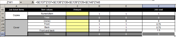
The result table collects the values for all job ticket items from the concerning column in the job ticket table.
It is recommended to use the IF function for each new calculation: =IF ( logical_test, value_if_true, value_if_false ). If the logical_test is true, the job cost is calculated. Else, the calculation returns a default value. In this example: 9999.99.
You can use the functions of most categories in Microsoft Office Excel to create a calculation. You cannot use the functions of category "Database".
The reduction of the price for a certain amount of [Copies] is taken from the [Copies table] in the "Utilities" worksheet.
The formula syntax and usage of the VLOOKUP function is described in the Microsoft Excel help file.
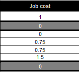
The value in Z3 is returned to the customer.
You must test each new formula for correctness.